Rough Volatility

Overview

Rough volatility explores recent developments in volatility process modeling. Research has suggested that volatility is more appropriately replicated by a process whose paths are “rougher” than Brownian motion.

TLDR

★★★★/5
Genre: Academic Writing
Highlights: Fractional Brownian Motion, Hedging VIX Options, Early Chapters
Drawbacks: Highly theoretical, Inaccessible for Traders

Notes

In general, we assume that log prices take the form:

dY_t = \mu_t dt + v_tdW_t

Where:

$v_t$ is constant for Black-Scholes
$v_t = \sigma(Y_t,t)$ for Dupire’s local volatility model

In rough volatility, we model $\log v_t$ using Fractional Brownian Motion (fBm) or $W_t^H$ , where $H \in (0,1)$ .

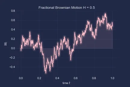
The primary difference between Bm and fBm is that the increments need not be independent. fBm is a Gaussian process $B_H(t)$ , which has $E(B_H(t)) = 0$ and has the following covariance function:

E[B_H(t)B_H(s)] = \frac{1}{2}(|t|^{2H} + |s|^{2H} - |t-s|^{2H})

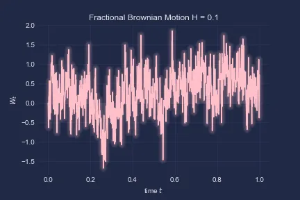
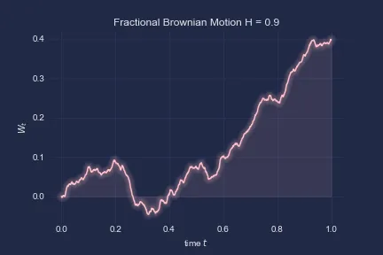
Note that for $H = \frac{1}{2}$ , we recover traditional Bm. For higher $H$ , we observe higher positive correlation of the increments.

Let’s explore some simulations of fBm:

def fbm_cholesky(H, n, T):
    t = np.linspace(0, T, n)
    dt = t[1] - t[0]

    cov_matrix = np.zeros((n, n))
    for i in range(n):
        for j in range(i, n):
            cov_matrix[i, j] = 0.5 * (abs(t[i])**(2*H) + abs(t[j])**(2*H) - abs(t[i]-t[j])**(2*H))
            cov_matrix[j, i] = cov_matrix[i, j]

    # jitter since numerical errors make matrix not positive definite
    cov_matrix += np.eye(n) * 1e-10
    L = np.linalg.cholesky(cov_matrix)

    Z = np.random.normal(size=n)
    W = np.dot(L, Z)

    return W, t

Standard Brownian Motion: fBm

The fitted range of $H$ parameters used are “0.08-0.2”: fBm

Finally, the smoothest case: fBm

Rough Fractional Stochastic Volatility (RFSV)

The main model specified in the text is the RSFV which is defined by the solution to the following SDE:

dX_t = vdW_t^H - \alpha (X_t -m)dt

This model is favourable for a few reasons:

It is stationary, and the OU process allows for a long reversion time scale
Inference methods for an OU process and fBm are well known

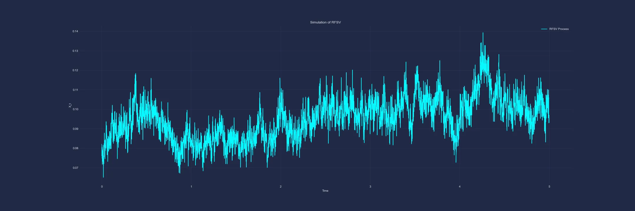
Now let’s visualise this model by using a Euler-Marayama approximation. First, discretising the SDE:

X_{n + 1} = X_n + v(W_{n+1}^H - W_n^H) - \alpha (X_n - m) \Delta t

Let’s implement this in Python:

W, t = fbm_cholesky(H, N, T)
X = np.zeros(N)
X[0] = mu
dW = np.diff(W)

for i in range(1, N):
    X[i] = X[i-1] + alpha * (m - X[i-1]) * dt + v * dW[i-1]

Recall that we are modeling log-variance. With the below parameter selection, we observe:

$v = 0.3$
$X_0 = m = -4$ (starting point and reversion center-point)
$H = 0.14$
$T = 5$
$\alpha = 5 * 10^{-4}$ (Reversion extremity)

Options Trading Under rBergomi

In chapter two, they discuss a practical application of the rough volatility model to options prices and demonstrate that one can effectively fit the SPX volatility smile with very few parameters- $H, \nu$ and $Q$ . Although there are few parameters, it seems they lack intuition/resolution on their specific role in curve fitting and are best tuned through ‘guessing and checking’. The curve fits the market decently well, but there are issues with extreme-call skew and retreating specific subsections of the smile appears to be impractical. A different position-based retreat scheme may be necessary for HFT market makers employing the technique- perhaps a correlated per-strike volatility adjustment would do the trick?

I also wonder about the practical application of slope change rates… Although we can change the ATM skew, how does the model fare with adjusting the convexity of smaller wings- say, the 10-15 delta calls and puts? For a bank, with less granular fitting requirements, this model may be sufficient, particularly for illiquid markets allowing some degree of interpolation between expiries for wing pricing. These questions are, in general, an issue with parameterised models for high-frequency market makers, which lack the flexibility to allow for big pricing adjustments due to excess supply/demand or risk management.

Market Impact

I found the chapter on market impact to be particularly interesting although less relevant for volatility modeling. The discussions around metaorders and the impact of the execution process are, although mathematically dense, rather intuitive. A Hawkes process is not something I had seen before reading this paper, but defining it as a generalization of the Poisson process is helpful. There is also a considerable amount of discussion around the idea that the market is endogenous- i.e. most orders are sent in reaction to other orders and have no economic motivation. This is very much the case for a lot of liquid instruments, for which a large proportion of the volume in the order book is market-maker flow, who place and delete orders using a reactive base-price and show quotes to facilitate liquidity. As such, I think it is a perfectly fair assumption to make.

Key Jargon:

Hawkes Process: a self-exciting point process
Convolution Product: the integral of the product of two functions

Rough Heston

Recall that the Heston Model is defined as follows:

\begin{aligned} \frac{dS_t}{dS_t} &= \sqrt{V_t}dB_t \\ dV_t &= \lambda(\theta - V_t)dt + \nu \sqrt{V_t}dW_t \end{aligned}

Where volatility is modeled by an OU process, with $\lambda$ the mean-reversion speed, $\theta$ the long-term variance level and $\nu$ the vvol. The main idea discussed in this chapter is replacing regular Brownian motion with an fBm process.

There exists some discussion of the so-called ‘Zumbach Effect’, which at a high level is the property that past squared returns forecast futures volatilities better than past volatilities forecast futures squared returns.

Hedging Under Rough Volatility

The main thing that caught my eye in this chapter was the notion that we can implement complex hedging or pricing strategies that are computationally expensive and speed up their execution by several orders of magnitude using deep learning. This could be useful, particularly for complex models built for pricing American options.

Conclusion

To me, a lot of the ‘meat’ of the text is in the first few chapters in which the authors introduce fBm as a new paradigm in stochastic volatility modeling. I particularly enjoyed section 6.3 Hedging VIX options: Empirical analysis- perhaps due to the familiar presentation of hedging strategy evaluations. The authors were certainly not wrong when they prescribed the readings as a prerequisite to a thorough understanding of this book, but I would also say with some high-level understanding of stochastic calculus- namely Brownian Motion, Stochastic Differential Equations and an introductory level of stochastic analysis- one can literally read between the lines and gauge a lot of the key ideas. Interestingly, I found the articles with higher ratios of text:latex to be the more actionable ones; it was difficult to hang on in the latter parts of the book like Chapter 5, 7, 9 and 10 which were particularly notation heavy. Chapter 9 of the text also introduced diamond trees and forests, which was not something I had seen before.

Things I didn’t understand

Riccati Equations
Volterra Equations
Stochastic Convolution Equations- it seems this may be the sum of two or more stochastic processes, but I’m not certain…
Most of the “Rough Affine Models” chapter. It seems this chapter is the culmination of the splashes of mathematics that was unclear to me throughout the entire book. It could be interesting to revisit in a year from now, following more studies of stochastic analysis.
The Brownian Semi-Stationary Process

Things worth exploring

It seems that the idea that at-the-money skew in US markets can be well modeled using a power-law function of time to expiry is a quite commonly accepted idea in academia. It would be interesting to see if this model fits HK implied volatilities.

\psi(\tau) = A\tau^{-0.4}

Through reading this text I stumbled upon a nice database for historical realized vols in different indices: the Oxford-Man Institute of Quantitative Finance Realized Library. It seems to be discontinued, but some people posted old versions online. The Schema can be found here.
Zero-Intelligence Realized Variance Estimation is referenced within the text, and from a skim of the abstract appears to have an interesting discussion of historical reazlied volatility measures.