Recurrent Neural Networks: Visualizing Hidden Activations

Introduction

In this blog post, we’ll delve into Recurrent Neural Networks (RNNs) by solving a simple prediction task and visualizing the hidden unit activations. This approach will provide insights into how the network learns and represents information internally.

The Problem

Our task is to train an RNN to predict the next character in a sequence of the form $a^nb^n$ or $a^nb^nc^n$, where $n$ is a positive integer. Specifically:

1. For $a^nb^n$: The sequence consists of $n$ ‘a’s followed by $n$ ‘b’s.
2. For $a^nb^nc^n$: The sequence consists of $n$ ‘a’s, followed by $n$ ‘b’s, followed by $n$ ‘c’s.

In these sequences, all characters after the last ‘a’ are deterministic. For example, given the input “aaab”, the network should predict the next character as ‘b’ with probability 1.

Recurrent Neural Networks: A Brief Overview

Recurrent Neural Networks are a class of artificial neural networks designed to process sequential data. Unlike feedforward networks, RNNs have connections that form directed cycles, allowing them to maintain an internal state or “memory”. This makes them particularly well-suited for tasks involving time series or sequence prediction.

The basic structure of an RNN can be described by the following equations:

$$\begin{aligned} h_t &= f(W_{hx}x_t + W_{hh}h_{t-1} + b_h) \\ y_t &= g(W_{yh}h_t + b_y) \end{aligned}$$

Where:

• $x_t$ is the input at time step $t$
• $h_t$ is the hidden state at time step $t$
• $y_t$ is the output at time step $t$
• $W_{hx}$, $W_{hh}$, and $W_{yh}$ are weight matrices
• $b_h$ and $b_y$ are bias vectors
• $f$ and $g$ are activation functions (typically non-linear)

This recursive formulation allows RNNs to process sequences of arbitrary length, making them ideal for our character prediction task.

$a^nb^n$ Simple Recurrent Network

For the $a^nb^n$ problem, we construct an SRN with 2 input units, 2 hidden units, and 2 output units. After training for 100,000 epochs, we achieve an impressively low error rate of 0.0129. Let’s visualize the hidden activations to understand how the network solves this task:

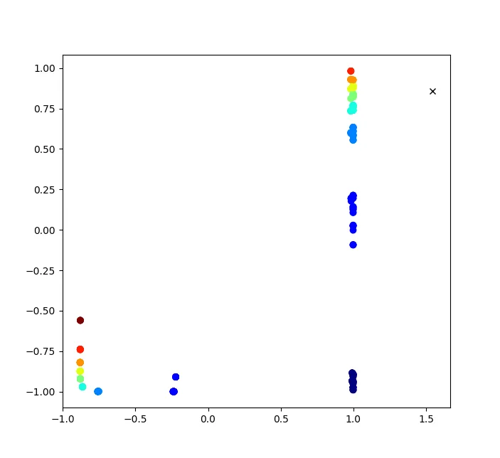
The activation space reveals two distinct clusters:

1. A cluster parallel to the x-axis, corresponding to ‘a’ characters.
2. A cluster at the top of the plot, corresponding to ‘b’ characters.

These clusters serve dual purposes:

1. They distinguish between ‘a’ and ‘b’ classes.
2. Variations within each cluster encode count information.

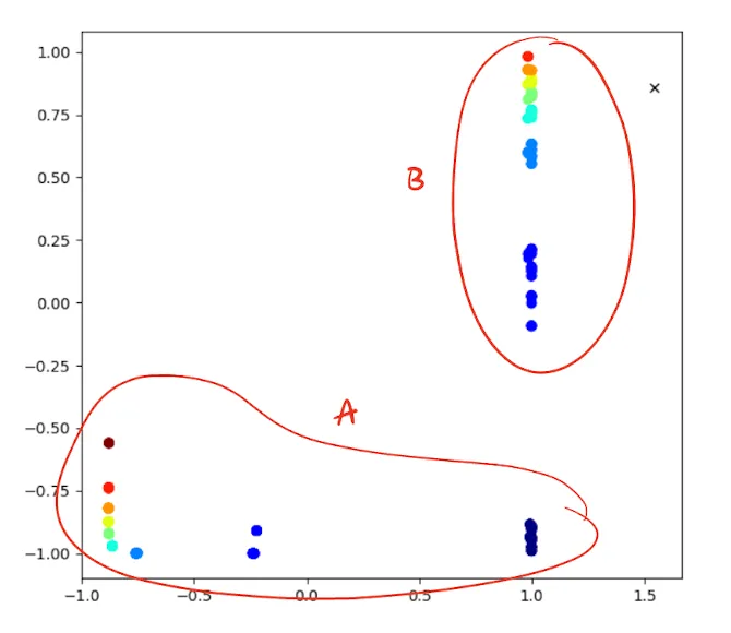
We can interpret the activations as follows:

• For ‘a’ characters: A more negative x-value indicates a higher count of ‘a’s seen so far. Interestingly, after the 4th ‘a’, the trend shifts upward instead of continuing left.
• For ‘b’ characters: A more positive y-value indicates a higher count of ‘b’s expected to follow.

As the network processes a string of ‘a’s and ‘b’s, it traverses this activation space in a clockwise manner. Notably, all deterministically predictable entries (the first ‘a’ after a sequence of ‘b’s and all ‘b’ entries) roughly align along the line x = 1. Other points can only be predicted probabilistically.

$a^nb^nc^n$ Simple Recurrent Network

Extending our problem to three dimensions, we now consider sequences of the form $a^nb^nc^n$. Our network architecture expands to 3 input units, 3 hidden units, and 3 output units. After 200,000 epochs of training, we achieve an error rate of 0.0083.

Let’s visualize the 3-dimensional hidden activations:

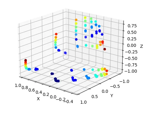
Remarkably, many insights from the 2D case generalize to 3D. We observe four main clusters:

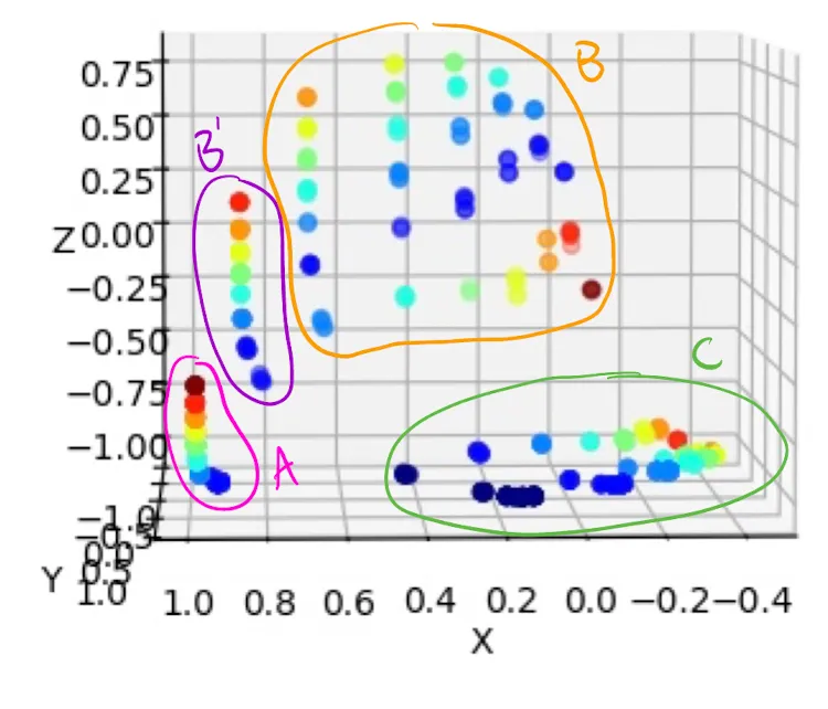
1. Cluster A: Contains non-deterministic ‘a’s.
2. Cluster B’: A transition state containing the first deterministic ‘b’ in a sequence.
3. Cluster B: Approximately aligns with Y = -1, containing remaining ‘b’s and the transition ‘c’.
4. Cluster C: Approximately aligns with Z = -1, containing remaining ‘c’s and the transition ‘a’.

As in the 2D case, we can conceptually separate deterministic and non-deterministic points. The network traverses this 3D space in an organized manner: A → B’ → B → C → A.

Each cluster acts as a counter, with different positions within a cluster representing the number of remaining characters of that type. For a clearer view of this counting mechanism:

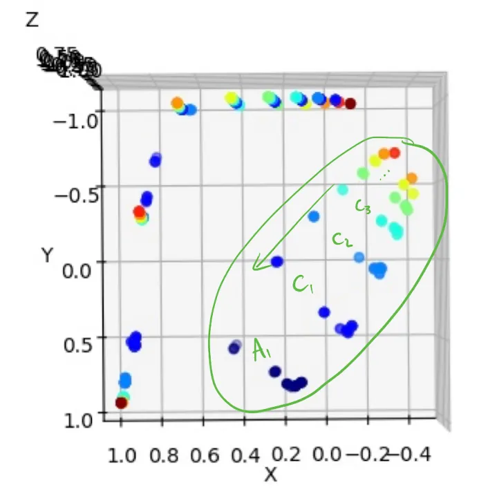
Here, $A_1$ represents the end of a ‘c’ sequence and the first ‘a’ of the next sequence, while $C_n$ indicates n ‘c’s remaining. This monotonic counting vector is present in all clusters, and viewing from the perspective of the previous figure, we move through all clusters in a clockwise fashion.

Conclusion

By visualizing the hidden activations of RNNs trained on $a^nb^n$ and $a^nb^nc^n$ sequences, we’ve gained valuable insights into how these networks internally represent and process sequential information. The emergent structure in the activation space demonstrates the network’s ability to learn both classification and counting tasks simultaneously, showcasing the power and interpretability of RNNs in sequence prediction tasks.