Arithmetic Asian Tail Options

Introduction

Asian options are a class of path-dependent exotic options whose payoff depends on the average price of the underlying asset over a certain period during the option’s life, rather than solely on the price at maturity. Specifically, arithmetic Asian options calculate the average using the arithmetic mean of the asset prices at predetermined intervals. This averaging feature reduces the option’s susceptibility to extreme price movements, making them particularly appealing in volatile markets where price manipulation near expiration is a concern.

However, pricing arithmetic Asian options presents significant challenges due to the lack of a closed-form analytical solution. Under the Black-Scholes framework, the underlying asset price is modeled as a geometric Brownian motion, implying that asset prices are lognormally distributed. While this assumption allows for analytical solutions for standard European options, the arithmetic average of lognormal variables does not follow a known distribution, complicating the valuation process. This has led to the development of various numerical and analytical approximation methods aimed at accurately pricing and hedging these options.

Several key unique methodologies have emerged in the literature, not limited to the following list:

• Monte Carlo Simulation with Control Variates: A numerical method that enhances the efficiency of Monte Carlo simulations by reducing variance, thereby improving pricing accuracy
• Geman-Yor Laplace Transform Approach: An analytical technique utilizing Laplace transforms to derive pricing formulas for Asian options, particularly effective for options with continuous averaging
• Rogers-Shi Partial Differential Equation (PDE) Method: A PDE approach that provides bounds and approximations for the option price, offering insights into the option’s behavior

In this blog post, we will delve into Monte-Carlo methodologies, exploring their theoretical foundations and practical implementations. Finally, in a numerical analysis in Python, we aim to illustrate its effectiveness and limitations, providing a comprehensive understanding of pricing and hedging arithmetic Asian options.

Theoretical Framework

Let $(\Omega, \mathcal F, \{\mathcal F_t\}_{t\geq 0}, \mathbb P)$ be a filtered probability space satisfying the usual conditions of completeness and right-continuity. In the Black-Scholes framework, under the risk-neutral measure $\mathbb Q$, equivalent to the real-world measure $\mathbb P$, the discounted price process of the underlying asset follows a geometric Brownian motion:

$$dS_t = rS_tdt + \sigma S_tdW_t^{\mathbb Q}$$

Where $r$ is the constant risk-free rate, $\sigma > 0$ is the constant volatility, and $W_t^{\mathbb Q}$ is a standard Brownian motion under $\mathbb Q$. An arithmetic Asian option’s payoff depends on the arithmetic average of the underlying asset’s price over some period. If we consider continuous averaging over the interval $[0,T]$, the arithmetic average is defined as:

$$A_T = \frac{1}{T} \int_0^T S_tdt$$

For a European-style arithmetic Asian call option with strike price $K$, the payoff $V$ is defined as:

$$V = (A_T - K)^+$$

The goal of this blog post is to determine the fair price of the arithmetic Asian call option $C$ as $t = 0$, which is defined as:

$$C = e^{-rT} \mathbb E^{\mathbb Q}[V|\mathcal F_0] = e^{-rT} \mathbb E^{\mathbb Q}[(A_T - K)^+]$$

Monte Carlo with Control Variates

Monte Carlo methods are a suite of numerical tools used for evaluating expectations, typically used when closed-form solutions are unavailable or intractable. However, standard Monte Carlo simulations can be computationally expensive. Control variates offer a way to reduce this variance, increasing the efficiency and accuracy of the simulation.

Standard Monte Carlo typically consists of the following steps:

1. Generate $M$ independent paths of the asset price process
2. For each of the simulated paths, calculate a corresponding payoff
3. Approximate the expected value by taking a sample average over all paths
4. Simulation of Asset Price Paths

Let us consider a standard geometric Brownian motion:

$$S_t = S_0 \exp \left( \left(r - \frac{\sigma^2}{2}\right)t + \sigma W_t\right)$$

We discretise the time interval $[0,T]$ into N partitions of equal length $\Delta t = T/N$ such that we can computationally evaluate the following approximation:

$$S_{t_{i+1}} = S_{t_i} \exp\left (\left(r - \frac{\sigma^2}{2}\right)\Delta t + \sigma \sqrt{\Delta t} Z_i \right)$$

Where $Z_i \sim \mathcal N(0,1)$ are independent standard normal variables.

For each simulated path, we compute the arithmetic average $A_T$:

$$A_T = \frac{1}{N} \sum_{i - 1}^N S_{t_i}$$

Finally, the estimated options price is the average of discounted payoffs over $M$ simulated paths:

$$\hat C = e^{-rT} \frac{1}{M}\sum_{j=1}^M (A_T^{(j)} - K)^+$$

Where $A_T^{(j)}$ is the arithmetic average of the $j$-th simulated path.

It is important to note that the path generation step in Monte Carlo should not be limited to Geometric Brownian motion (GBM). While GBM assumes continuous paths and constant volatility, real-world asset prices often exhibit features like jumps, stochastic volatility and mean-reversion that GBM does not capture.

As an improvement, we can consider Jump-Diffusion models, which introduce discontinuities to paths governed by a Poisson process or stochastic volatility models where the dynamics of volatility are governed by an Ornstein-Uhlenbeck process. In the interest of conciseness these methods will not be explored in this blog post.

Variance Reduction in Monte Carlo

The central limit theorem states that the estimation error of $\hat C$ is normally distributed with standard deviation proportional to $\frac{1}{\sqrt{M}}$.

$$\begin{align*} Var(\hat C) &= Var \left(\frac{1}{M} \sum_{j = 1}^M V^{(j)} \right) \\ &= \frac{1}{M^2} \sum_{j = 1}^M Var (V^{(j)}) \\ &= \frac{1}{M^2} M \sigma^2 \\ &= \frac{\sigma^2}{M} \\ \therefore SE(\hat C) &= \frac{\sigma}{\sqrt{M}} \end{align*}$$

Where $\sigma$ is the standard deviation of the samples, samples are i.i.d., and SE is the standard error of the estimator.

While basic the Monte Carlo estimator is unbiased, it has a relatively slow order of convergence ($\mathcal O(\frac{1}{\sqrt{N}})$). As demonstrated above, this property is a direct consequence of the i.i.d. condition of the samples and is grounded in the Law of Large Number and the Central Limit Theorem. Variance reduction techniques aim to decrease this variance without introducing bias. One example of this is the use of control variates.

The control variate method leverages the known expected value of a correlated variable to reduce the variance of the estimator. Let $Y$ be the random variable representing the payoff of the arithmetic Asian option, and $X$ be a control variate with known expectation. We define the adjusted estimator as:

$$\hat Y_{CV} = \hat Y + \beta (\mathbb E (X) - \hat X)$$

Where $\beta$ is a coefficient to be determined. The optimal value of $\beta$ that minimises the variance of $\hat Y_{CV}$ is:

$$\beta^* = \frac{Cov(Y,X)}{Var(X)}$$

This quantity is typically unknown, so it can be estimated from the simulated data. The variance of the control variate estimator can be calculated as follows:

$$\begin{align*} Var(\hat Y_{CV}) &= Var\left( \hat Y + \beta (\mathbb E (X) - \hat X)\right) \\ &= Var(\hat Y) + \beta^2 Var(\hat X) - 2\beta Cov(\hat Y, \hat X) \\ &= Var(\hat Y) + \left( \frac{Cov(\hat Y, \hat X)}{Var(\hat X)}\right)^2 Var(\hat X) - 2 \left( \frac{Cov(\hat Y, \hat X)}{Var(\hat X)}\right) Cov(\hat Y, \hat X) \\ &= Var(\hat Y) - \frac{Cov(\hat Y, \hat X)^2}{Var(\hat X)} \\ &= Var(\hat Y ) - Var(\hat Y) \rho_{\hat X \hat Y}^2 \\ &= Var(\hat Y) (1 - \rho_{\hat X \hat Y}^2) \end{align*}$$

Hedging and Greeks Calculation

In options trading, calculating the Greeks is crucial for risk management and devising hedging strategies. One practical approach to estimate Greeks within the Monte Carlo framework is the finite difference method. This method involves perturbing input parameters slightly and observing the resulting change in the estimated option price.

For instance, to compute Delta, which measures the sensitivity of the option price to changes in the underlying asset price, we can use a central finite difference approximation:

$$\Delta \approx \frac{C(S_0 + \delta S) - C(S_0 - \delta S)}{2\, \delta S}$$

A similar process can be used to calculate all first-order greeks. For higher-order Greeks like Gamma ($\Gamma$) we can use a second-order finite difference:

$$\Gamma \approx \frac{C(S_0 + \delta S) - 2C(S_0) + C(S_0 - \delta S)}{(\delta S)^2}$$

While straightforward, the finite difference method requires running additional simulations for each perturbed parameter value, which can be computationally intensive.

Numerical Experiments, Comparative Analysis & Conclusions

In this section, we compare the effectiveness of three different Monte Carlo simulation methods for pricing an arithmetic Asian option:

1. Crude Monte Carlo (CMC) Method
2. Control Variate with European Option (CV-Euro)
3. Control Variate with Geometric Asian Option (CV-Geo)

Our objective is to evaluate the accuracy and efficiency of these methods by analyzing their option price estimates and the associated standard errors as the number of simulations increases.

Simulation Parameters

The following parameters were used in the simulations:

• Initial Stock Price ($S_0$): $100
• Strike Price ($K$): $100
• Time to Maturity ($T$): 1 year
• Risk-Free Rate ($r$): 0%
• Volatility ($\sigma$): 20%
• Number of Time Steps ($n$): 252 (daily observations)
• Number of Simulations ($M$): 1,000; 5,000; 10,000; 50,000; 100,000

Results

The option price estimates and standard errors for each method are summarized in the following table:

Simulations	Crude Price	Crude SE	CV Euro Price	CV Euro SE	CV Geo Price	CV Geo SE
1,000	4.409092	0.226160	4.490657	0.129479	4.599432	0.005753
5,000	4.455136	0.101448	4.629808	0.058475	4.595136	0.002664
10,000	4.529010	0.072266	4.631864	0.040899	4.596585	0.001918
50,000	4.570938	0.032661	4.618924	0.018314	4.595519	0.000849
100,000	4.590457	0.023119	4.614984	0.012976	4.595743	0.000604

Analysis of Results

Convergence of Option Prices:

• All methods converge towards a similar option price as the number of simulations increases
• The CV-Geo method consistently provides estimates closer to the true option price even with fewer simulations

Standard Error Reduction:

• The standard error decreases with an increasing number of simulations for all methods
• The CV-Geo method achieves the lowest standard errors across all simulation sizes, indicating superior variance reduction
• The CV-Euro method also reduces variance compared to the CMC method but is less effective than the CV-Geo method

Figures and Interpretation

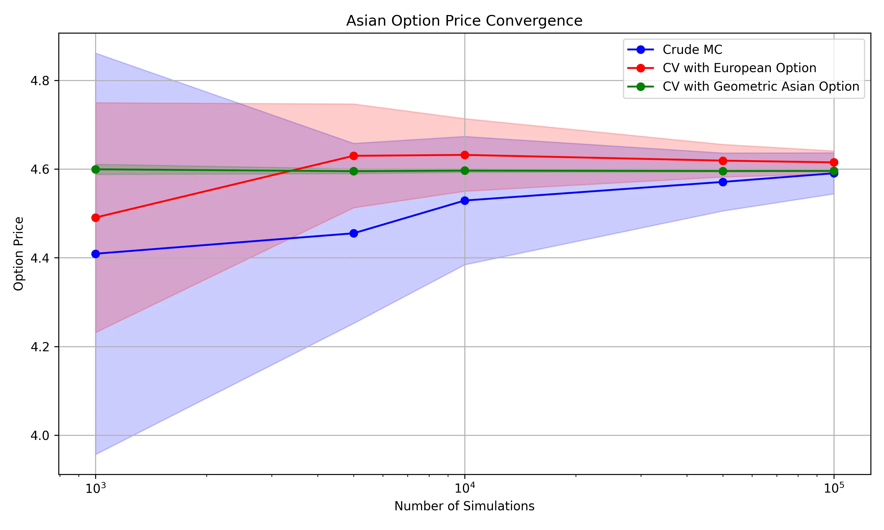
This figure plots the estimated option prices against the number of simulations on a logarithmic x-scale for all three methods. Shaded areas represent the confidence intervals (±2 standard errors).

• The CV-Geo method’s option price estimates stabilize quickly and remain within a narrow confidence interval even at lower simulation counts
• The CMC method shows significant fluctuation in option price estimates at lower simulations due to higher variance
• The CV-Euro method improves upon the CMC method but still exhibits wider confidence intervals compared to the CV-Geo method

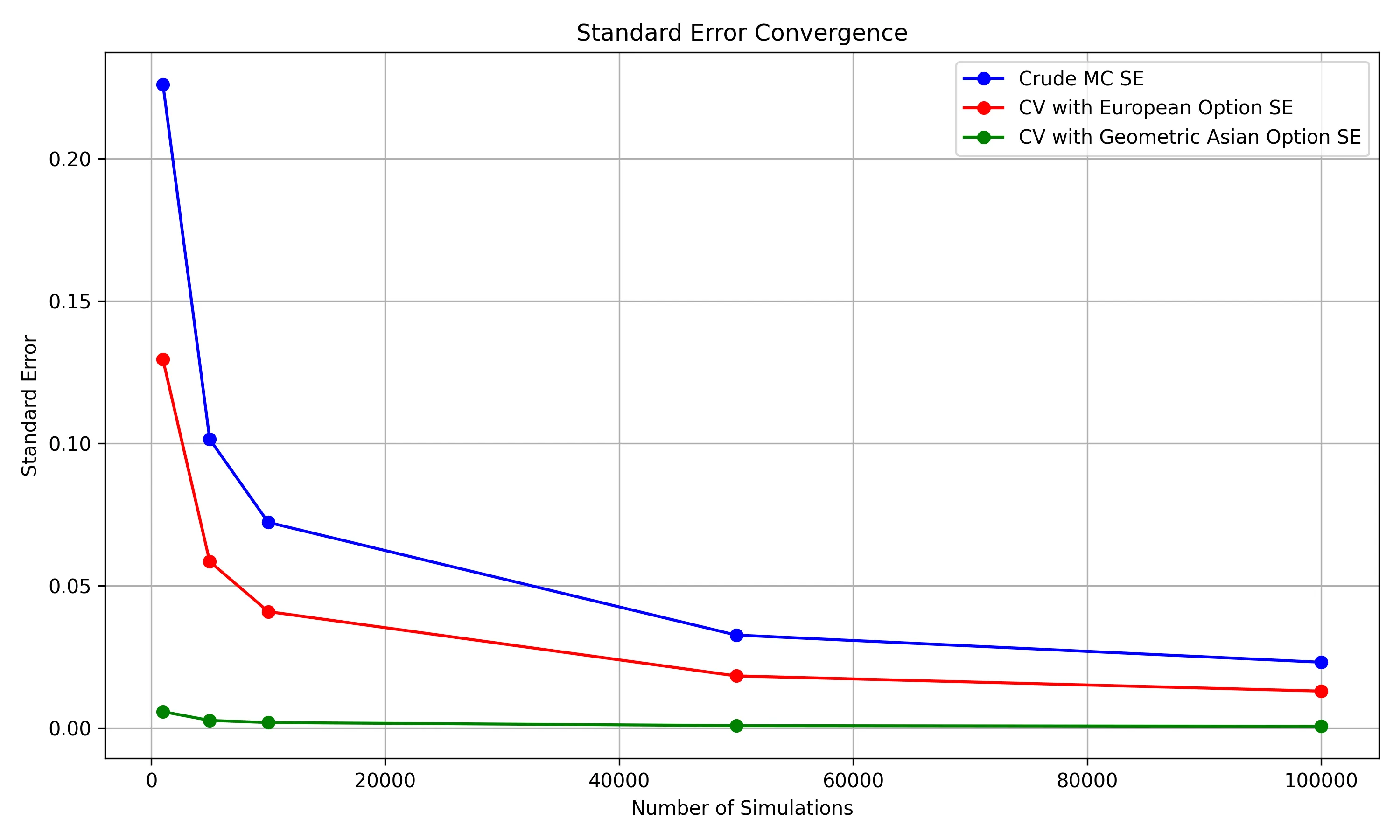
This figure displays the standard errors associated with each method’s option price estimates as the number of simulations increases.

• The CV-Geo method demonstrates the most rapid decrease in standard error, showcasing its efficiency in variance reduction. This makes sense, as the correlation between the geometric option and the arithmetic one is the highest
• The CV-Euro method also reduces standard error compared to the CMC method but at a slower rate than the CV-Geo method
• The CMC method exhibits the highest standard errors, indicating the need for a significantly larger number of simulations to achieve comparable accuracy

Conclusion

This comparative analysis highlights the effectiveness of using control variate techniques, particularly with the geometric Asian option, in pricing arithmetic Asian options via Monte Carlo simulation.

• Efficiency: The CV-Geo method significantly outperforms both the CMC and CV-Euro methods in terms of reducing variance and improving convergence speed
• Accuracy: With fewer simulations, the CV-Geo method provides highly accurate option price estimates with minimal standard error

Implications for Practice

Implementing the CV-Geo method can lead to more efficient pricing of complex financial derivatives, enabling traders and risk managers to make better-informed decisions with greater confidence in the results.

References

1. Boyle, P., Broadie, M., & Glasserman, P. (1997). Monte Carlo Methods for Security Pricing. Journal of Economic Dynamics and Control
2. Kleijnen, J. P., & Ridder, A. (2010). Variance Reduction Techniques in Monte Carlo Methods. Encyclopedia of Quantitative Finance